Headline result
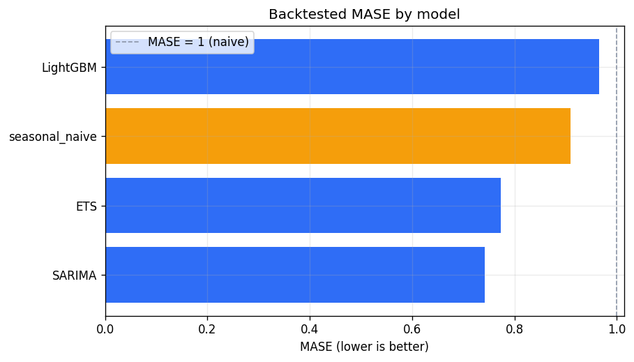
Mean across a 6-fold rolling-origin backtest, 28-day horizon.
- 0.74
- SARIMA MASE (1.00 = naive)
- −18.5%
- error vs seasonal-naive (MASE)
- −21%
- error vs seasonal-naive (sMAPE)
The target is total daily units sold by a UK online retailer (UCI Online Retail II, 739 days). The benchmark is a seasonal-naive forecast — last week's value, repeated. A SARIMA model beats it on every metric, not just the one that flatters it:
| model | sMAPE | RMSE | MASE | improvement vs naive |
|---|---|---|---|---|
| SARIMA | 29.67 | 6,982 | 0.741 | +18.5% |
| ETS | 30.63 | 7,174 | 0.773 | +15.0% |
| seasonal-naive | 37.73 | 8,105 | 0.910 | 0.0% |
| LightGBM | 36.77 | 8,502 | 0.966 | −6.1% |
The data, and why it's hard
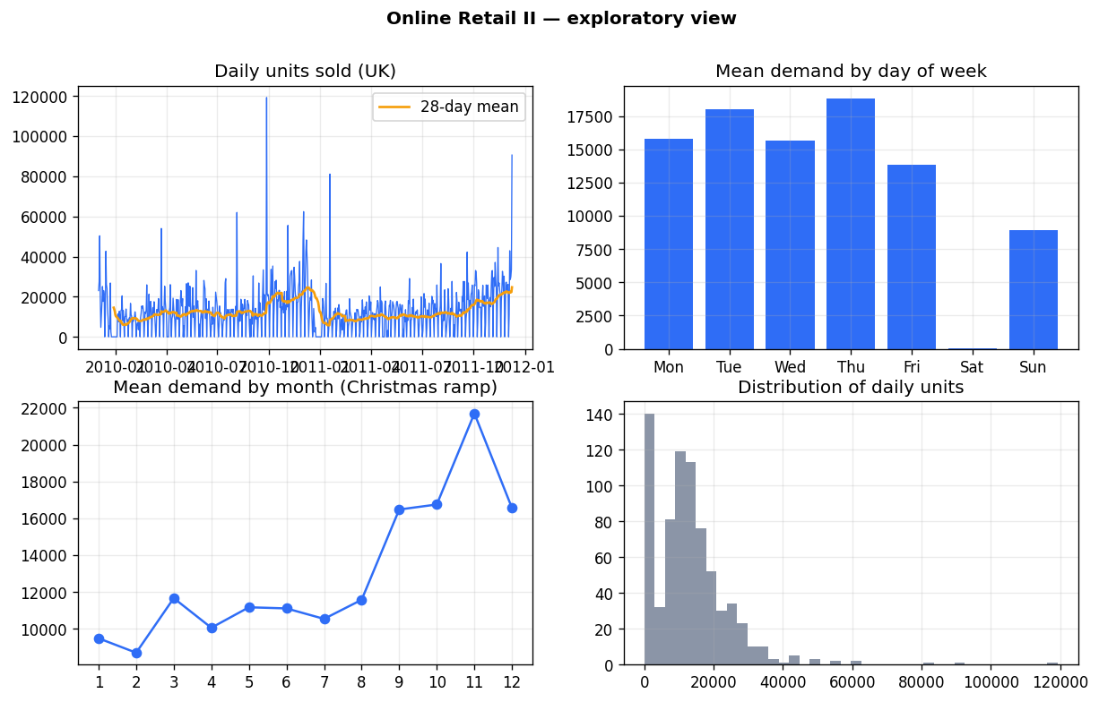
Aggregated to a daily series, the data has three features that decide the modelling:
- A hard weekly cycle. Saturday is a structural zero — the retailer doesn't process orders that day. I treat "closed on Saturday" as a business rule and force those forecasts to zero. The seasonal-naive baseline already gets this from the prior week, so applying the same rule to every model keeps the comparison honest.
- A Christmas ramp. Volume builds into November and December, the retailer's peak.
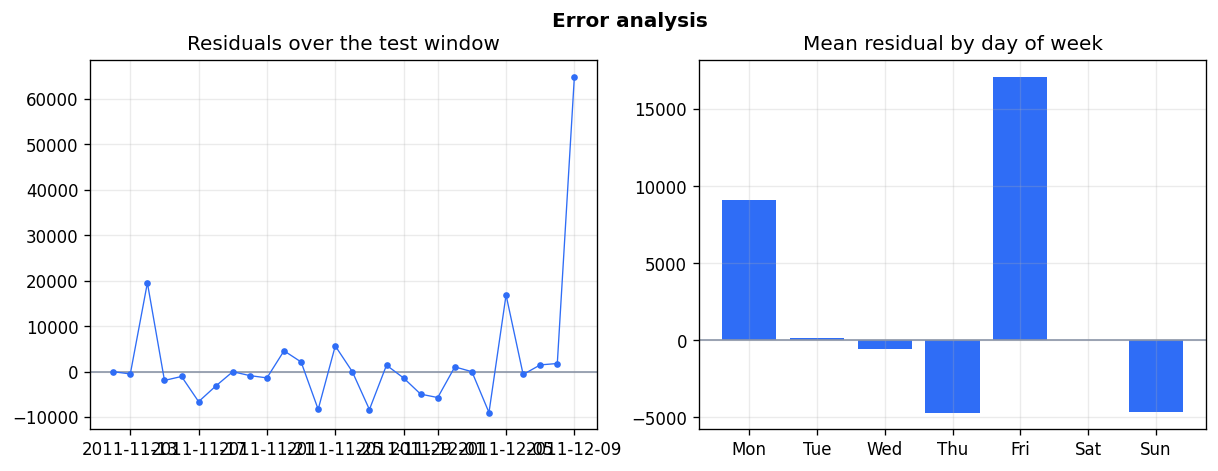
- Heavy tails. Occasional large wholesale orders make the daily series spiky (coefficient of variation 0.86 daily vs 0.44 weekly). Those spikes are the bulk of the remaining error.
How it's evaluated
Time-based, no leakage, lift measured against an explicit baseline.
Every model is scored with rolling-origin cross-validation: six consecutive 28-day windows, each model trained only on the data before its window. No shuffling, no peeking. The headline metric is MASE — mean absolute error scaled by the in-sample seasonal-naive error — because it is comparable across series and states the improvement over the benchmark directly (MASE < 1 means you beat it).
The ML model (LightGBM on lag, rolling, and calendar/holiday features, forecast recursively) is the interesting honest result: it does not beat the classical seasonal models on this single rigid-weekly series. That's expected — gradient boosting earns its keep across many series with a global model, not on one smooth aggregate where a well-specified SARIMA is hard to beat. Reporting that is the point.
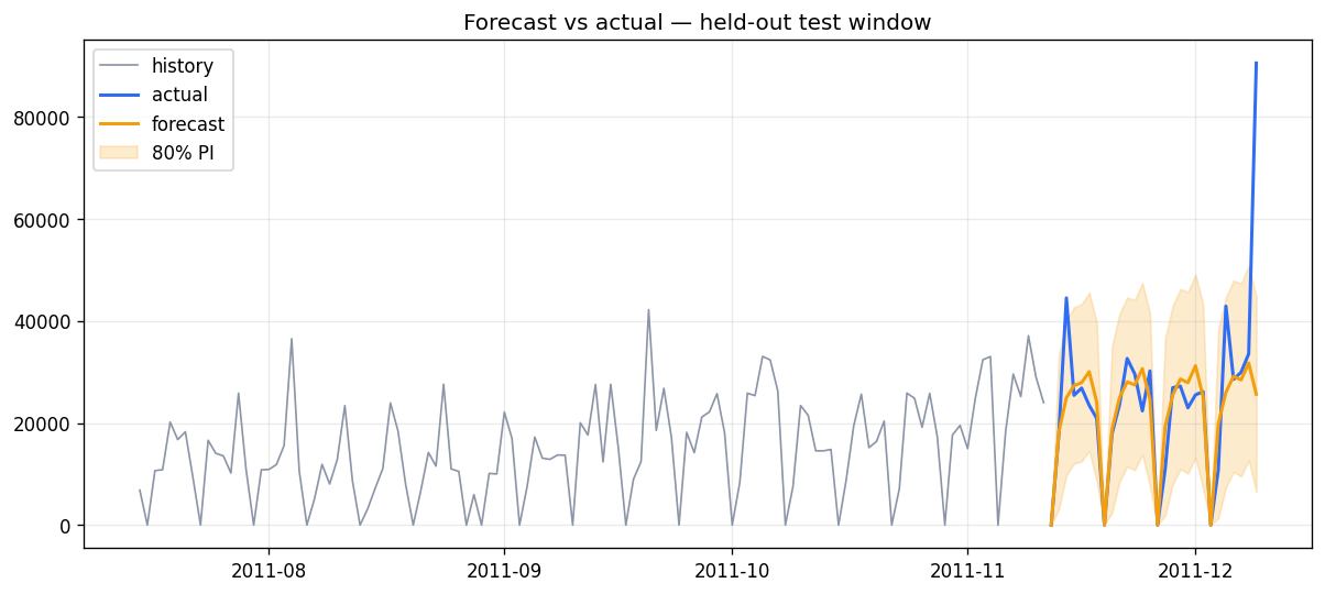
Forecast and error analysis
Causal bonus: recovering a promo effect
Difference-in-differences, checked against a known ground truth.
There's no labelled promotion in the data, so I simulate one and check the estimator. A synthetic 24-store × 180-day panel is built from the real demand shape — shared seasonality, store-level scaling, noise — and a known +15% uplift is applied to treated stores in the post period. A two-way fixed-effects difference-in-differences on log demand (store fixed effects absorb level, date fixed effects absorb the common seasonal movement) recovers the truth:
- +15%
- injected uplift (ground truth)
- +14.9%
- DiD estimate
- ±0.7pp
- 95% CI [14.2%, 15.6%]
The validation states the method, recovers a known answer, and reports the interval.
Reproduce it
Public data (no Kaggle auth), deterministic, one command. The download script pulls Online Retail II straight from UCI; raw data is never committed.
pip install -r requirements.txtpython run.py— downloads, backtests, writes every figure and the metrics reportpytest -q— 26 tests (metrics, feature-leakage, baselines, backtest, DiD)